LANDMARK Outputs and Visualization Guide

This page details the structure and content of the two main output files produced by LANDMARK, explains how to interpret their attributes, and gives best practices for their visualization in a GIS (e.g., QGIS).

---

Overview

LANDMARK outputs two vector GeoPackage files (.gpkg):

• Slopelines (thalweg network):
  slopelines_se_HSO_<input_name>.gpkg

• Ridgelines (ridge network):
  ridgelines_se_HSO_<input_name>.gpkg

Each file contains a layer of LineString features, representing individual segments of the extracted networks, with associated attributes.

---

1. Slopelines (Thalweg Network)

Description

The slopelines file contains segments representing the primary drainage lines (thalwegs) identified in the DEM. Each segment connects two consecutive drainage points along the calculated flow network. These lines correspond to pathways of surface water concentration and potential channelization.

Key Attributes

Field	Type	Description
id_ch	int	Unique ID of the current slopeline segment.
start_pnt	int	ID of the segment’s upstream (start) point.
end_pnt	int	ID of the segment’s downstream (end) point.
id_ch_out	int	ID of the next downstream segment.
id_ch_main	int	ID of the main downstream segment in the hierarchy.
A_out	int	Contributing area at the start point (in map units², e.g., m²).
length	float	Segment length (in spatial units, e.g., meters).
sso	int	Stream Segment Order (internal topological order).
hso	int	Horton/Strahler stream order of the segment.
slope_pct	float	Slope between endpoints (%). (if computed)
curvature	float	Vertical curvature at start point. (if computed)

Important Filtering Tips

• For QGIS visualization:
  Due to network complexity, filter the displayed lines for clarity.

  • Recommended filter:

    • A_out: Only show segments with a large enough contributing area (e.g., A_out > 10000). This emphasizes main channels and removes tiny tributaries.

    • hso: Show segments with high stream order (e.g., hso >= 5) to display the main drainage skeleton.

  • A_out is generally the most effective filter for thalwegs, as it directly corresponds to hydrological significance.

Geomorphological Attributes

If computed, slope_pct and curvature fields provide additional information for landform and hydrological analysis (e.g., highlighting steep or concave/convex channel segments).

---

2. Ridgelines (Ridge Network)

Description

The ridgelines file contains segments forming the primary ridge network—divides or crests separating drainage basins. Each segment connects two consecutive ridge points and corresponds to lines of maximum elevation divergence.

Key Attributes

Field	Type	Description
id_rdl	int	Unique ID of the ridgeline to which the segment belongs.
start_pnt	int	ID of the segment’s start ridge point.
end_pnt	int	ID of the segment’s end ridge point.
length	float	Segment length (in spatial units, e.g., meters).
jun_el	int	Index of the first junction (node) on the ridgeline.
A_spread	float	Spread area: approximates the lateral area controlled by the ridge (m²).
slope_pct	float	Slope between endpoints (%). (if computed)
curvature	float	Vertical curvature at start point. (if computed)

Important Filtering Tips

• For QGIS visualization:
  To avoid clutter, filter ridgelines using:

  • A_spread: Show only segments with large enough spread area (e.g., A_spread > 10000). This highlights the main ridges and omits minor, local divides.

Geomorphological Attributes

Fields slope_pct and curvature, if present, allow further morphometric analysis (e.g., identifying steep or curved ridges).

---

Practical Tips for GIS Visualization

• Filtering in QGIS:

  • Open the GeoPackage layer, go to the attribute table, and use the “Select by Expression” tool to filter features (e.g., A_out > 5000 or A_spread > 10000).

  • You can symbolize lines by stream order (hso) or spread area (A_spread) for clearer maps.

• Display Recommendations:

  • For an overview, use strict thresholds to show only the main network skeleton.

  • For detailed studies (e.g., small catchments), lower thresholds to display more features.

• Attribute Calculation Notes:

  • Slope and curvature are only included if you enabled the corresponding option during processing.

  • Spatial units (meters, m²) depend on the CRS of your DEM.

Example Outputs and Visualization in QGIS

Below are examples of QGIS visualizations illustrating different filtering options and map styles using the output GeoPackages from LANDMARK.

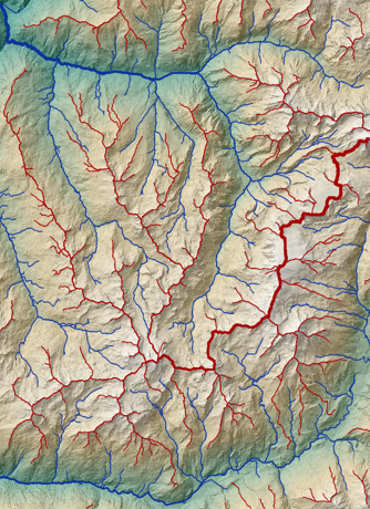
LiDARHD 5 m DEM. Drainage and dispersion areas filtered at \(10^6\) m². The width of the blue (thalweg) and red (ridge) lines is proportional to the corresponding area.

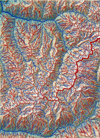
LiDARHD 5 m DEM. Drainage and dispersion areas filtered at \(10^5\) m².

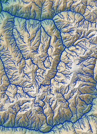
LiDARHD 5 m DEM. Thalweg network filtered by Horton order > 4. The width of the blue lines is proportional to the Horton order of each segment.